Research

What does an applied mathematician do?

Applied mathematicians see the world through problems and solutions. For example, we like to encode questions like

"How does heat flow through a metal rod?"

as problems like

"Find a smooth function u(x,t) which satisfies the heat equation [∂/∂t - ∂²/∂x²]u(x,t)=0 and initial condition u(x,0)=u₀(x) and boundary conditions u(0,t)=h₀(t) and u(1,t)=h₁(t)."

where the functions u₀, h₀, h₁ are known data. The solution of this problem, the function u, is supposed to represent the temperature of the rod at position x along its length from 0 to 1 at time t after initial time 0. While a physicist or engineer may be interested in the modelling assumptions required to ensure that such a problem can be used to accurately answer the original question, a mathematician becomes interested only after the problem has been derived.

The above problem is called an "initial boundary value problem", because the problem specifies information about the initial value of a function and its behaviour on the boundaries. Not all applied mathematicians study initial boundary value problems, but they are a popular format of problem among those who work in the field of partial differential equations.

An applied mathematician can engage with a problem such as the above in a variety of ways, including:

Discern qualitative features of the solution. Consider the following argument. The partial differential equation (PDE) above has the feature that the time derivative is set up to balance out the second spatial derivative. This means that the PDE "dislikes" solutions with high spatial curvature; as time increases, a plot of the spatial dependence of the solution should get closer to a straight line. The boundary conditions say that the straight line should pass through 0 at both x=0 and x=1, so the solution u(x,t) must approach the line U(x)=0 as time t increases. This was achieved without actually solving the original problem, but still gives some information about the solution. One very important property that can be studied in this way is "wellposedness", the questions of whether there exists a unique solution to a given problem, and whether a small change in the data will have a correspondingly small effect on the solution.
Find a numerical approximation of the solution. A given partial differential equation can be approximated by a difference equation so that its solution may be found approximately using a computer. There are a variety of difference equation approximations and numerical schemes that may be employed, to various effect. More advanced approximation methods may yield better approximations to the solution, but may be overkill for simpler problems. The properties of the particular problem at hand tend to have significant impact on which numerical schemes are effective and which are not.
Obtain an exact analytical representation of the solution. There are many problems where this is impossible, but for some problems, including the example above, it can be done. The most widely known method for the above problem is separation of variables, solution of Sturm-Liouville problem (a smaller, easier problem than the original problem) and expansion in eigenfunctions. The result is a formula for the solution as a Fourier series, so this method is often called the Fourier series method (FSM). There are other methods for solving the same problem, including the unified transform method (UTM), which results in a complex contour integral representation of the solution.
Analyse solution methods. The above problem has several fundamentally different solution methods, so mathematicians are interested in understanding what makes them work, how the same methods could be applied to other similar problems, and why one method might be better" than the other (and what the word "better" should mean in this context!). Mathematicians are also interested in attempting to adapt a known method to problems that are a little less similar, to understand how the method might break down or to grasp a deeper interpretation of how the method works. This often includes extension to problems that have no physical motivation, but are mathematically interesting for the ways they interact with methods.
Analyse solution representations. The unique solution of the above problem has two fundamentally different representations. At which of those one might arrive depends upon the method used, but even the solution representations may have different utility. The solution of a problem such as that above cannot be expressed using the standard library of mathematical functions such as polynomials, trigonometric and exponential functions, hence the use of a series or an integral, which are different kinds of infinite sums. In practice, to plot the solution, one can only use finitely many terms in such infinite sums (or it would take forever!), so one truncates the infinite to finite sums. One might ask "how many terms does it take for the truncation to approximate the actual value of the infinite sum to a certain degree?" and compare the results for different solution representations. Different solution representations can also have varying utility in other applications, such as understanding the behaviour of the solution in different asymptotic limits: "what happens if I make the metal rod shorter but also more resistant at a certain rate, and which solution representation gives me a clearer understanding of this process?"

I tend to be drawn to problems for which 1 is too easy and, because 3 is possible, 2 is mostly useful for formulating hypotheses. Therefore, I usually engage with problems in senses 3–5. Much of my work is dedicated to analysing UTM, and its application to solving an ever expanding class of problems. Often this represents the first time that any analytic solution representation has been obtained for a given problem, which makes the comparative and contrastive aspects of 5 difficult, so I focus a little more on senses 3–4 than 5.

Examples of Dave's research

Analytic solution of IBVP

An initial boundary value problem (IBVP) is a problem stated with a PDE, an initial condition (IC) and several boundary conditions (BC), such as the above problem for the heat equation. Although the problem described above may be solved by an undergraduate student, what might appear to be a relatively minor complication to the problem may make it much more difficult to solve.

Consider the following apparatus.

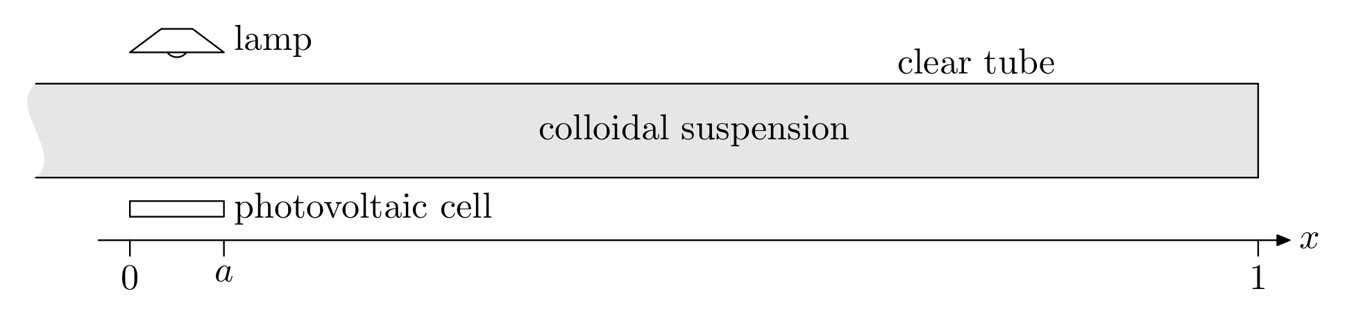
The clear tube contains a colloidal suspension in which the suspensurate has nonhomogenous concentration, and suppose that the opacity of the liquid depends upon suspensurate concentration in a simple way. If a physical scientist wants to know the concentration of the suspensurate at horizontal position x and time t, then the lamp and photovoltaic cell could be used to measure the concentration at x=0, thereby specifying a BC, and an IBVP may be set up to describe diffusion. As diffusion is described using the same model as heat flow, the heat equation serves as the PDE, and an IC may be determined from the initial state of the system. The problem with this model is that the measurement of opacity is not taken exactly at x=0 (even a very expensive photovoltaic cell must have finite width!) so the experimentalist cannot hope to measure concentration at x=0, but only an average concentration near x=0. This replaces the BC with a nonlocal condition, making the IBVP (or, rather, INVP) much more difficult.

Although this problem had been studied through approach 2 since the 1960's, my work with Miller was the first successful solution in the sense of 3. In the same paper, we also employed approach 4 by describing UTM's applicability to a much broader class of INVP. A further achievement of [MS2018a] was the clearest statement in the scientific record of the general algorithm and applicability criteria of UTM.

In an earlier work with Pelloni [PS2018a], we provided the extension of UTM to general initial multipoint value problems (IMVP). For problems of second spatial order, the solution representation was given explicitly, and wellposedness was determined. For problems of third spatial order, wellposedness was assumed and a solution representation provided. The algorithm was described for higher order problems. An alternative version of the UTM algorithm, also suitable for IMVP, was provided in [MS2018a]. The two methods were contrasted and their respective realms of superior applicability elucidated.

Analysis of UTM

My thesis [Smi2011a] and first paper [Smi2012a] provide the general applicability of UTM to IBVP, including a proof that it may be used to solve all wellposed problems, and to decide wellposedness of IBVP. In the more recent trilogy [FS2016a], [PS2016a], [Smi2015a] we expound the success of UTM in terms of a transform and inverse transform pair, and of a new species of spectral object, augmented eigenfunctions.

The famous pseudoeigenfunctions represent discrete "approximate eigenfunctions" in the sense that the norms of their remainder functionals are individually controlled by some small ε and provide a richer spectral representation of differential operators, leading to improved numerical techniques. In contrast, augmented eigenfunctions are families of objects parametrised by a continuous complex variable, the eigenvalue, satisfying the requirement that a complex contour integral of the remainder functional, with respect to the eigenvalue and against a Fourier type kernel, converges to zero. So an individual augmented eigenfunction need not be a good approximation of an eigenfunction, but the approximation appears in the collective.

If, a little optimistically, eigenfunctions are thought of as the basis in which a linear operator is diagonalised, then the Fourier transform's diagonalisation of differential operators explains the appearance of eigenfunctions in FSM, and the value of this method for solving IBVP. The problem is that there are myriad degenerate irregular spatial differential operators arising in well posed IBVP, where the eigenfunctions are hopelessly far from forming a basis. UTM does not deal in a true diagonalisation of the spatial differential operator because the transform expresses the problem in terms of augmented eigenfunctions. However, and this is the crucial advantage of UTM, augmented eigenfunctions are a diagonalisation plus a remainder which, upon application of the inverse transform, vanishes. Therefore, in conjunction with the inverse transform, the transform to augmented eigenfunctions is as good as diagonalising the spatial differential operator. With augmented eigenfunctions understood, it reasonable to claim that activity 4 is complete for UTM as applied to IBVP.

Interface problems

Interface problems are often used to model phenomena in which there is a physical divide transition between different media in which different physical laws apply. For example, one may see an interface between water and air, or between two metals of different conductivity. Interfaces may be allowed to move in time (such as the water surface due to waves) or may be fixed by mechanical constraints. The more variation allowed in the interface the more complicated the problem.

In [SS2015a], we studied how heat flows through complex networks of metal rods. We were able extend the unified transform method to various prototypical configurations of metal rods, each with arbitrary conductivity and finite or infinite length, to find explicit solution representations in terms of complex contour integrals. For a simple star shaped network of three rods, we plotted how the temperature at each point in each rod varies in time.

The more theoretical paper [DSS2016a] studies interface problems for the third order linearised KdV equation. Here, there is not such a clear physical interpretation to use for intuition on which problems ought to be wellposed, so we derived criteria for wellposedness in terms of precisely which version of the equation is specified on each side of the interface and on the algebraic form of the interface conditions. We consider rather general linear interface conditions at a fixed interface, with half line domains on either side of the interface. Beyond establishing wellposedness, we also solve the initial interface problem explicitly via an extension of UTM, and discuss further generalisations.